It is hard to imagine that anyone who lived during the Great Depression was not profoundly affected by it. From the beginning of the Depression in 1929 to the time the economy hit bottom in 1933, real GDP plunged nearly 30%. Real per capita disposable income sank nearly 40%. More than 12 million people were thrown out of work; the unemployment rate soared from 3% in 1929 to 25% in 1933. Some 85,000 businesses failed. Hundreds of thousands of families lost their homes. By 1933, about half of all mortgages on all urban, owner-occupied houses were delinquent (Wheelock, 2008).
The economy began to recover after 1933, but a huge recessionary gap persisted. Another downturn began in 1937, pushing the unemployment rate back up to 19% the following year.
The contraction in output that began in 1929 was not, of course, the first time the economy had slumped. But never had the U.S. economy fallen so far and for so long a period. Economic historians estimate that in the 75 years before the Depression there had been 19 recessions. But those contractions had lasted an average of less than two years. The Great Depression lasted for more than a decade. The severity and duration of the Great Depression distinguish it from other contractions; it is for that reason that we give it a much stronger name than “recession.”
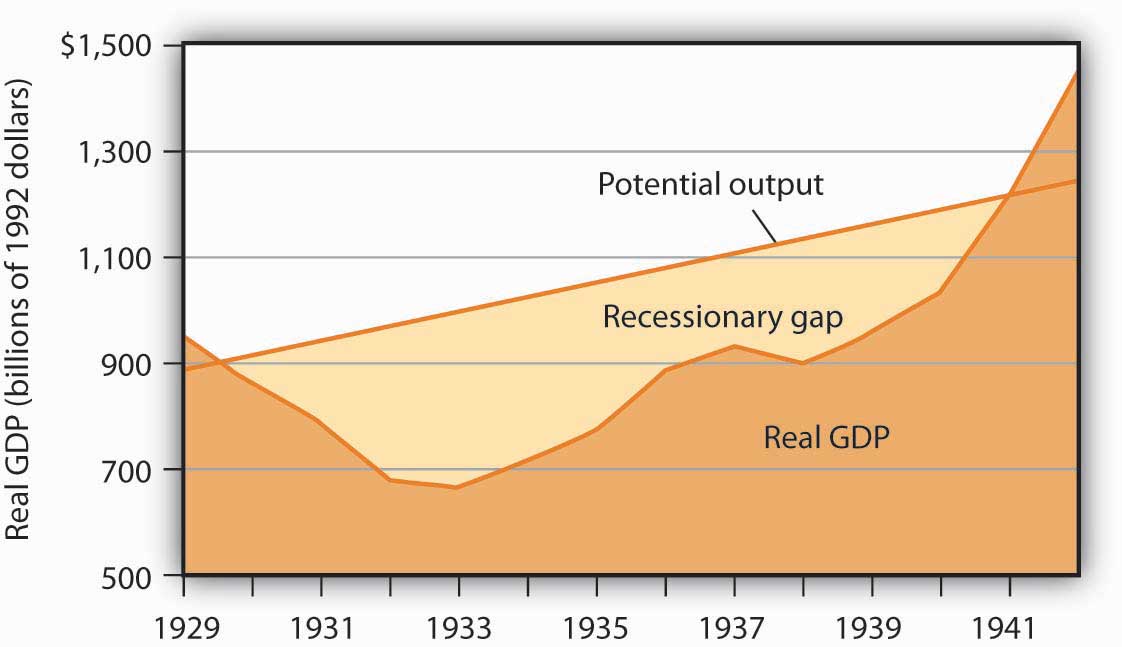
Figure 17.1 “The Depression and the Recessionary Gap” shows the course of real GDP compared to potential output during the Great Depression. The economy did not approach potential output until 1941, when the pressures of world war forced sharp increases in aggregate demand.
Figure 17.1 The Depression and the Recessionary Gap

The dark-shaded area shows real GDP from 1929 to 1942, the upper line shows potential output, and the light-shaded area shows the difference between the two—the recessionary gap. The gap nearly closed in 1941; an inflationary gap had opened by 1942. The chart suggests that the recessionary gap remained very large throughout the 1930s.
The Great Depression came as a shock to what was then the conventional wisdom of economics. To see why, we must go back to the classical tradition of macroeconomics that dominated the economics profession when the Depression began.
Classical economics is the body of macroeconomic thought associated primarily with 19th-century British economist David Ricardo. His Principles of Political Economy and Taxation, published in 1817, established a tradition that dominated macroeconomic thought for over a century. Ricardo focused on the long run and on the forces that determine and produce growth in an economy’s potential output. He emphasized the ability of flexible wages and prices to keep the economy at or near its natural level of employment.
According to the classical school, achieving what we now call the natural level of employment and potential output is not a problem; the economy can do that on its own. Classical economists recognized, however, that the process would take time. Ricardo admitted that there could be temporary periods in which employment would fall below the natural level. But his emphasis was on the long run, and in the long run all would be set right by the smooth functioning of the price system.
Economists of the classical school saw the massive slump that occurred in much of the world in the late 1920s and early 1930s as a short-run aberration. The economy would right itself in the long run, returning to its potential output and to the natural level of employment.
In Britain, which had been plunged into a depression of its own, John Maynard Keynes had begun to develop a new framework of macroeconomic analysis, one that suggested that what for Ricardo were “temporary effects” could persist for a long time, and at terrible cost. Keynes’s 1936 book, The General Theory of Employment, Interest and Money, was to transform the way many economists thought about macroeconomic problems.
In a nutshell, we can say that Keynes’s book shifted the thrust of macroeconomic thought from the concept of aggregate supply to the concept of aggregate demand. Ricardo’s focus on the tendency of an economy to reach potential output inevitably stressed the supply side—an economy tends to operate at a level of output given by the long-run aggregate supply curve. Keynes, in arguing that what we now call recessionary or inflationary gaps could be created by shifts in aggregate demand, moved the focus of macroeconomic analysis to the demand side. He argued that prices in the short run are quite sticky and suggested that this stickiness would block adjustments to full employment.
Keynes dismissed the notion that the economy would achieve full employment in the long run as irrelevant. “In the long run,” he wrote acidly, “we are all dead.”
Keynes’s work spawned a new school of macroeconomic thought, the Keynesian school. Keynesian economics asserts that changes in aggregate demand can create gaps between the actual and potential levels of output, and that such gaps can be prolonged. Keynesian economists stress the use of fiscal and of monetary policy to close such gaps.
The experience of the Great Depression certainly seemed consistent with Keynes’s argument. A reduction in aggregate demand took the economy from above its potential output to below its potential output, and, as we saw in Figure 17.1 “The Depression and the Recessionary Gap”, the resulting recessionary gap lasted for more than a decade. While the Great Depression affected many countries, we shall focus on the U.S. experience.
The plunge in aggregate demand began with a collapse in investment. The investment boom of the 1920s had left firms with an expanded stock of capital. As the capital stock approached its desired level, firms did not need as much new capital, and they cut back investment. The stock market crash of 1929 shook business confidence, further reducing investment. Real gross private domestic investment plunged nearly 80% between 1929 and 1932. We have learned of the volatility of the investment component of aggregate demand; it was very much in evidence in the first years of the Great Depression.
Other factors contributed to the sharp reduction in aggregate demand. The stock market crash reduced the wealth of a small fraction of the population (just 5% of Americans owned stock at that time), but it certainly reduced the consumption of the general population. The stock market crash also reduced consumer confidence throughout the economy. The reduction in wealth and the reduction in confidence reduced consumption spending and shifted the aggregate demand curve to the left.
Fiscal policy also acted to reduce aggregate demand. As consumption and income fell, governments at all levels found their tax revenues falling. They responded by raising tax rates in an effort to balance their budgets. The federal government, for example, doubled income tax rates in 1932. Total government tax revenues as a percentage of GDP shot up from 10.8% in 1929 to 16.6% in 1933. Higher tax rates tended to reduce consumption and aggregate demand.
Other countries were suffering declining incomes as well. Their demand for U.S. goods and services fell, reducing the real level of exports by 46% between 1929 and 1933. The Smoot–Hawley Tariff Act of 1930 dramatically raised tariffs on products imported into the United States and led to retaliatory trade-restricting legislation around the world. This act, which more than 1,000 economists opposed in a formal petition, contributed to the collapse of world trade and to the recession.
As if all this were not enough, the Fed, in effect, conducted a sharply contractionary monetary policy in the early years of the Depression. The Fed took no action to prevent a wave of bank failures that swept the country at the outset of the Depression. Between 1929 and 1933, one-third of all banks in the United States failed. As a result, the money supply plunged 31% during the period.
The Fed could have prevented many of the failures by engaging in open-market operations to inject new reserves into the system and by lending reserves to troubled banks through the discount window. But it generally refused to do so; Fed officials sometimes even applauded bank failures as a desirable way to weed out bad management!
Figure 17.2 Aggregate Demand and Short-Run Aggregate Supply: 1929–1933
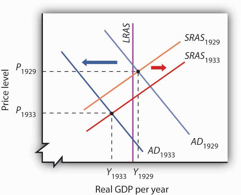
Slumping aggregate demand brought the economy well below the full-employment level of output by 1933. The short-run aggregate supply curve increased as nominal wages fell. In this analysis, and in subsequent applications in this chapter of the model of aggregate demand and aggregate supply to macroeconomic events, we are ignoring shifts in the long-run aggregate supply curve in order to simplify the diagram.
Figure 17.2 “Aggregate Demand and Short-Run Aggregate Supply: 1929–1933” shows the shift in aggregate demand between 1929, when the economy was operating just above its potential output, and 1933. The plunge in aggregate demand produced a recessionary gap. Our model tells us that such a gap should produce falling wages, shifting the short-run aggregate supply curve to the right. That happened; nominal wages plunged roughly 20% between 1929 and 1933. But we see that the shift in short-run aggregate supply was insufficient to bring the economy back to its potential output.
The failure of shifts in short-run aggregate supply to bring the economy back to its potential output in the early 1930s was partly the result of the magnitude of the reductions in aggregate demand, which plunged the economy into the deepest recessionary gap ever recorded in the United States. We know that the short-run aggregate supply curve began shifting to the right in 1930 as nominal wages fell, but these shifts, which would ordinarily increase real GDP, were overwhelmed by continued reductions in aggregate demand.
A further factor blocking the economy’s return to its potential output was federal policy. President Franklin Roosevelt thought that falling wages and prices were in large part to blame for the Depression; programs initiated by his administration in 1933 sought to block further reductions in wages and prices. That stopped further reductions in nominal wages in 1933, thus stopping further shifts in aggregate supply. With recovery blocked from the supply side, and with no policy in place to boost aggregate demand, it is easy to see now why the economy remained locked in a recessionary gap so long.
Keynes argued that expansionary fiscal policy represented the surest tool for bringing the economy back to full employment. The United States did not carry out such a policy until world war prompted increased federal spending for defense. New Deal policies did seek to stimulate employment through a variety of federal programs. But, with state and local governments continuing to cut purchases and raise taxes, the net effect of government at all levels on the economy did not increase aggregate demand during the Roosevelt administration until the onset of world war (Brown, 1956). As Figure 17.3 “World War II Ends the Great Depression” shows, expansionary fiscal policies forced by the war had brought output back to potential by 1941. The U.S. entry into World War II after Japan’s attack on American forces in Pearl Harbor in December of 1941 led to much sharper increases in government purchases, and the economy pushed quickly into an inflationary gap.
Figure 17.3 World War II Ends the Great Depression
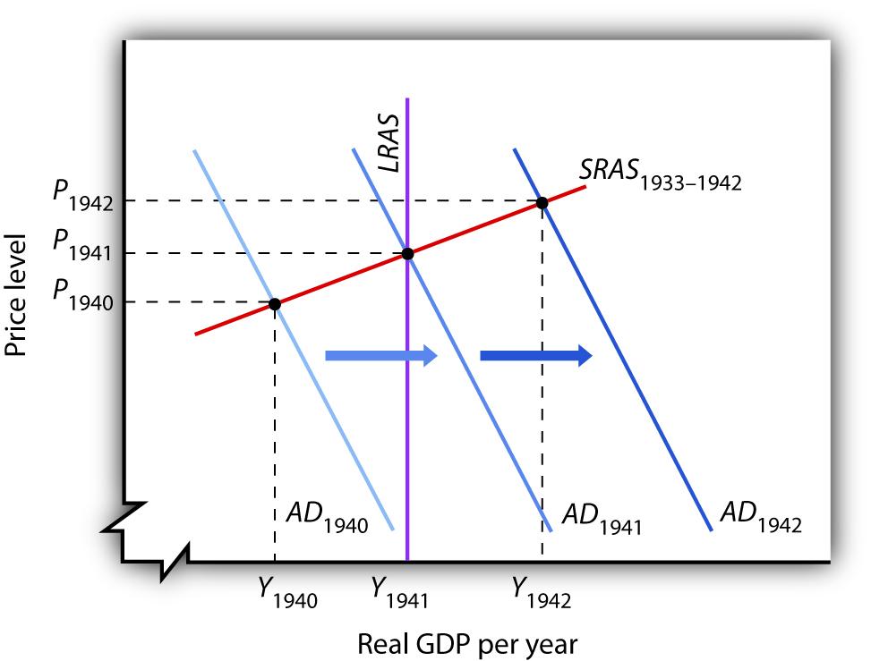
Increased U.S. government purchases, prompted by the beginning of World War II, ended the Great Depression. By 1942, increasing aggregate demand had pushed real GDP beyond potential output.
For Keynesian economists, the Great Depression provided impressive confirmation of Keynes’s ideas. A sharp reduction in aggregate demand had gotten the trouble started. The recessionary gap created by the change in aggregate demand had persisted for more than a decade. And expansionary fiscal policy had put a swift end to the worst macroeconomic nightmare in U.S. history—even if that policy had been forced on the country by a war that would prove to be one of the worst episodes of world history.
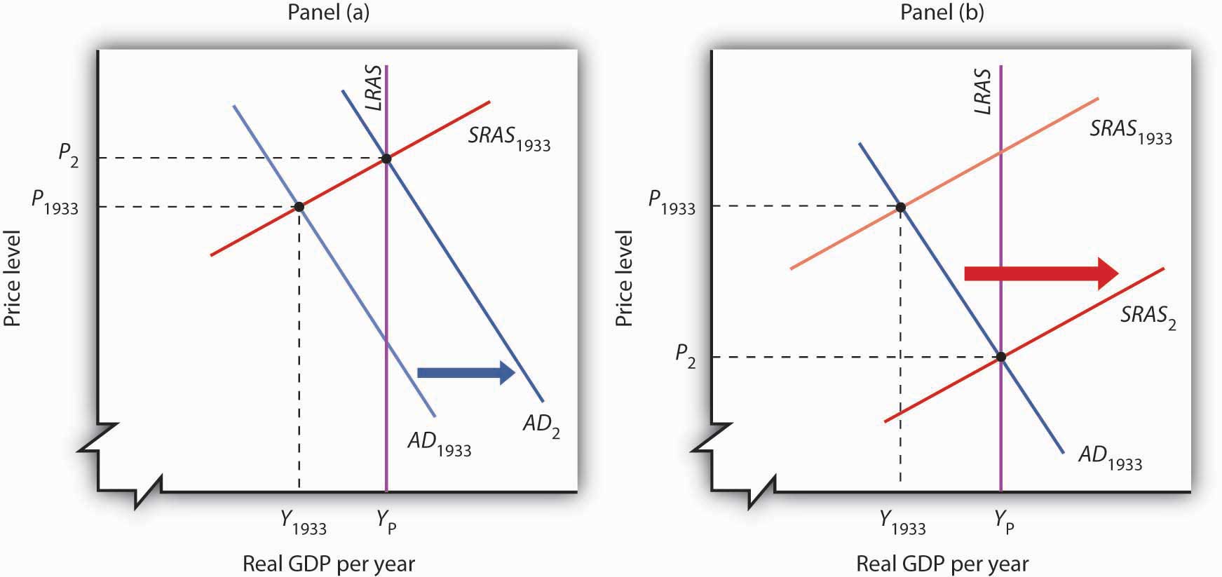
Imagine that it is 1933. President Franklin Roosevelt has just been inaugurated and has named you as his senior economic adviser. Devise a program to bring the economy back to its potential output. Using the model of aggregate demand and aggregate supply, demonstrate graphically how your proposal could work.

Although David Ricardo’s focus on the long run emerged as the dominant approach to macroeconomic thought, not all of his contemporaries agreed with his perspective. Many 18th- and 19th-century economists developed theoretical arguments suggesting that changes in aggregate demand could affect the real level of economic activity in the short run. Like the new Keynesians, they based their arguments on the concept of price stickiness.
Henry Thornton’s 1802 book, An Enquiry into the Nature and Effects of the Paper Credit of Great Britain, argued that a reduction in the money supply could, because of wage stickiness, produce a short-run slump in output:
“The tendency, however, of a very great and sudden reduction of the accustomed number of bank notes, is to create an unusual and temporary distress, and a fall of price arising from that distress. But a fall arising from temporary distress, will be attended probably with no correspondent fall in the rate of wages; for the fall of price, and the distress, will be understood to be temporary, and the rate of wages, we know, is not so variable as the price of goods. There is reason, therefore, to fear that the unnatural and extraordinary low price arising from the sort of distress of which we now speak, would occasion much discouragement of the fabrication of manufactures.”
A half-century earlier, David Hume had noted that an increase in the quantity of money would boost output in the short run, again because of the stickiness of prices. In an essay titled “Of Money,” published in 1752, Hume described the process through which an increased money supply could boost output:
“At first, no alteration is perceived; by degrees the price rises, first of one commodity, then of another, till the whole at least reaches a just proportion with the new quantity of (money) which is in the kingdom. In my opinion, it is only in this interval or intermediate situation … that the encreasing quantity of gold and silver is favourable to industry.”
Hume’s argument implies sticky prices; some prices are slower to respond to the increase in the money supply than others.
Economists of the 18th and 19th century are generally lumped together as adherents to the classical school, but their views were anything but uniform. Many developed an analytical framework that was quite similar to the essential elements of new Keynesian economists today. Economist Thomas Humphrey, at the Federal Reserve Bank of Richmond, marvels at the insights shown by early economists: “When you read these old guys, you find out first that they didn’t speak with one voice. There was no single body of thought to which everyone subscribed. And second, you find out how much they knew. You could take Henry Thornton’s 1802 book as a textbook in any money course today.”
Source: Thomas M. Humphrey, “Nonneutrality of Money in Classical Monetary Thought,” Federal Reserve Bank of Richmond Economic Review 77, no. 2 (March/April 1991): 3–15, and personal interview.
An expansionary fiscal or monetary policy, or a combination of the two, would shift aggregate demand to the right as shown in Panel (a), ideally returning the economy to potential output. One piece of evidence suggesting that fiscal policy would work is the swiftness with which the economy recovered from the Great Depression once World War II forced the government to carry out such a policy. An alternative approach would be to do nothing. Ultimately, that should force nominal wages down further, producing increases in short-run aggregate supply, as in Panel (b). We do not know if such an approach might have worked; federal policies enacted in 1933 prevented wages and prices from falling further than they already had.
Brown, E. C., “Fiscal Policy in the ’Thirties: A Reappraisal,” American Economic Review 46, no. 5 (December 1956): 857–79.
Wheelock, D. C., “The Federal Response to Home Mortgage Distress: Lessons from the Great Depression,” Federal Reserve Bank of St. Louis Review 90, no. 3 (Part 1) (May/June 2008): 133–48.